A JEPA world model that learns Mario by playing itself

01 · What we were trying to find out

Most successful Mario-playing programs are taught directly to play Mario. SethBling’s MarI/O evolves a NEAT network with a hand-coded fitness function over forward progress and survival; modern model-free RL agents define a reward and gradient-descend a policy against it. The model’s understanding of Mario — what a Goomba is, what gravity does, what comes after a pipe — is wired up implicitly through the action the agent eventually picks.

JEPA-style world models (Yann LeCun’s framing, Sobal et al.’s LeWorldModel recipe) promise a different decomposition: train an encoder + predictor self-supervised on game frames, then plan or train a policy on the frozen latents. The model first learns the dynamics — without reward, without action labels, without a goal — and only then is asked to do anything goal-directed with that knowledge.

Can you bootstrap a Mario-playing policy from a JEPA world model trained only on game frames and action labels — no rewards, no demonstrations, no game-specific engineering?

We’ve been building lemario, a from-scratch implementation of the LeWM recipe on NES Super Mario Bros, to find out. The representation side worked the first time. The control side took two structural redesigns and still hasn’t reached the flagpole. The most recent redesign — what this post is about — turned out to be necessary not because the system regressed, but because our measurement of whether the system regressed was too noisy to use. That is more interesting than the result it almost let us announce.

Here is what the system does on the real game today, after fifteen training iterations:

We framed the project around three hypotheses of increasing ambition. They organize the rest of this post:

• H1 — Stability. The LeWM single-regularizer recipe trains stably on Mario frames, without the exponential moving average, stop-gradient, pretrained backbone, or reconstruction loss that most self-supervised vision recipes lean on. If H1 fails, the recipe is too brittle to use on this kind of input at all, and the whole project is over.
• H2 — Structure. Frozen encoder features linearly probe to the game’s RAM-scraped physical quantities — x/y position, velocities, on-ground flag, is-dying flag. If H2 fails, the encoder is producing features without semantic content; anything we build on those features is operating on noise.
• H3 — Control. A planner or policy that consumes the frozen latents matches or exceeds MarI/O on level 1-1, and the same backbone generalizes zero-shot to held-out levels. This is the load-bearing claim — that self-supervised dynamics can substitute for hand-engineered fitness functions in a place where hand-engineered fitness functions are known to work.

H1 and H2 cleared on the first serious run, and we’ll dispatch them in one section. The rest of the post is the H3 story — what we tried, what failed, what we’re rebuilding before iter 16.

02 · The recipe — and a representation side that works

Before we get into what changed, it helps to say what a world model actually is in this context. The idea, in its modern form, is to learn a neural simulator of the environment from observation–action data: an encoder that maps the current observation to a compact representation, and a predictor that maps that representation plus an action to the next representation. Once it’s accurate enough, you can train a policy or run a planner inside the model instead of paying real-environment cost — and real-environment cost matters when one Mario episode is 1,500 frames the world model can simulate internally in milliseconds.

What distinguishes JEPA from earlier world-model recipes is where the predictor predicts. Most pre-JEPA approaches — Dreamer’s family of recurrent state-space models, MuZero’s tree-search models, the original world-models work — predict in some form of pixel space, either reconstructing the next frame or matching a learned pixel compression. JEPA predicts in latent space: the encoder produces a representation z, the predictor produces ẑ' for the next representation, and pixels never enter the prediction loss. The bet is that this skips the wasteful work of modeling every visual detail (every cloud, every grain of brick texture) and concentrates the model on whatever’s structurally important for the downstream task.

The hard part of any joint-embedding recipe is the collapse problem. An encoder and predictor trained jointly on a “predict the next latent” loss have a trivial degenerate solution: collapse every input to the same constant latent, and have the predictor output that constant. The loss goes to zero, the representations are useless, and nothing about the training-time signal tells you what just happened. All of the stabilization tricks in modern self-supervised vision — EMA-tracked target encoders (BYOL, DINO), stop-gradients between branches (SimSiam), momentum updates, pretrained backbones — exist to push the encoder away from this collapse without explicitly telling it to. Each one works; each one also couples training stability to an architectural choice that has nothing to do with the task. The LeWorldModel bet is that none of them is necessary: a single regularizer (SIGReg, which pushes the latent distribution toward an isotropic Gaussian-like shape via a covariance-style penalty) does the entire anti-collapse job by itself.

LeMario is built on that bet, and the constraints are load-bearing. SIGReg is the only regularizer. No exponential moving average of the encoder. No stop-gradient between encoder and predictor. No pretrained backbone. No reconstruction loss. If a stabilization trick from the broader SSL literature would help with something, we deliberately don’t use it — the whole point of the recipe is to find out what falls out when you don’t.

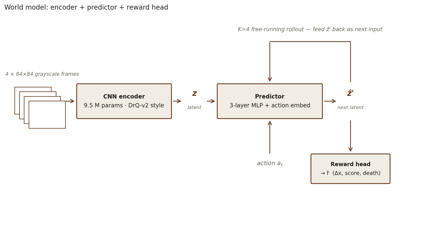
The pieces are small. A 9.5 M-parameter DrQ-v2-style CNN encoder turns a stack of four 84×84 grayscale frames (frame-stacking is the partial-observability remedy for an MDP with hidden velocity state) into a latent. A 3-layer MLP predictor, conditioned on a learned embedding of the action, predicts the next latent. Predictor training is free-running over K=4 steps: the predictor’s own output is fed back in as input for the next step, not the ground-truth encoded latent. This is the closest the model ever comes to an explicit dynamics loss, and it’s what keeps the encoder from discarding anything the predictor will need several frames downstream. The constraint isn’t theoretical — early single-step variants gave a vertical-velocity probe R² of 0.15, while the K=4 free-running variant pulled the same probe to 0.71. The encoder under single-step training had simply thrown away y-velocity, because the biased-random data didn’t make it locally necessary.

Trained on 2,000 right-biased-random trajectories of level 1-1 (621K frames, 26 GB on NVMe) with DDP across four 5090s, the recipe is stable: 60k steps, no divergence, no loss spikes once SyncBatchNorm and free-running training are both in place. After training, frozen encoder features linearly probe to the game’s internal RAM state at high fidelity: R² 0.71 on x_pos, 0.71 on y_vel, 0.98 on the on-ground flag, 1.00 on is-dying. The encoder, with no reward signal and no game-specific labels, has picked up enough physical state to recover the game’s hidden variables from the pixels alone.

That clears H1 and H2. The hard part — H3 — starts when you ask the latents to do something.

03 · The first attempt at control failed in an interesting way

The natural first thing to try with a frozen world model is model-predictive control: at each step, sample a few hundred candidate action sequences, roll each one out through the predictor, score them with a learned reward head, pick the best one, take the first action, repeat. This is the recipe behind everything from PETS to Dreamer’s planning baselines. We ran a dozen variants — varying horizon, planner prior, reward parameterization, multi-step vs single-step predictor training. The best one scored a mean x_pos of 790 over five episodes and 204 over ten. The worst was worse than standing still. None of them beat a hand-tuned biased-random sampler (mean x = 658) reliably.

The diagnostic that explained this came from a uniform-prior run. With the planner sampling all 12 buttons roughly equally and picking the highest-scoring trajectory, Mario literally stayed still on 9 of 10 episodes. The predictor had learned that “do nothing” trajectories are easy to predict and that prediction error is roughly proportional to motion. The reward head, trained on biased-random rollouts, then rewarded predictions it could trust — which were the ones where nothing moved.

This is the MSE predictability bias: a predictor trained to minimize mean-squared error in latent space prefers plans whose latents are predictable, not plans whose latents lead to high reward. The two objectives are aligned during pretraining because biased-random data covers both regimes. They come apart at planning time, because the planner can search over new plans the dataset didn’t contain — and the cheapest way to get a low-error prediction is to find a plan where almost nothing changes.

This isn’t a bug. It’s a property of the training objective. The fix isn’t a bigger model, a longer horizon, or a better planner — it’s training the predictor against something other than pure next-state error.

04 · The pivot: reward-augmented training and a closed-loop flywheel

We did two things in response — bolted a reward output onto the world model, and turned the whole training process into a loop.

Reward augmentation

The world model gets a second small head — a 3-layer MLP — that takes a predicted latent and emits a reward triple r̂: a forward-progress estimate Δx, a score-delta estimate, and a death flag. It trains jointly with the predictor on the cumulative corpus, MSE on each channel. Reward becomes a first-class output of the world model, not a post-hoc scoring function bolted on at planning time. The predictor now pays a loss when its imagined future is wrong about consequences, not just wrong about which pixels come next. The free-running K=4 rollout that’s been load-bearing throughout the project carries over unchanged: encoder, predictor, and reward head all see the multi-step constraint.

The closed-loop flywheel

Instead of a one-shot pretraining + planning pipeline, training becomes an iterative loop with the corpus, the world model, and the policy all updating in tandem.

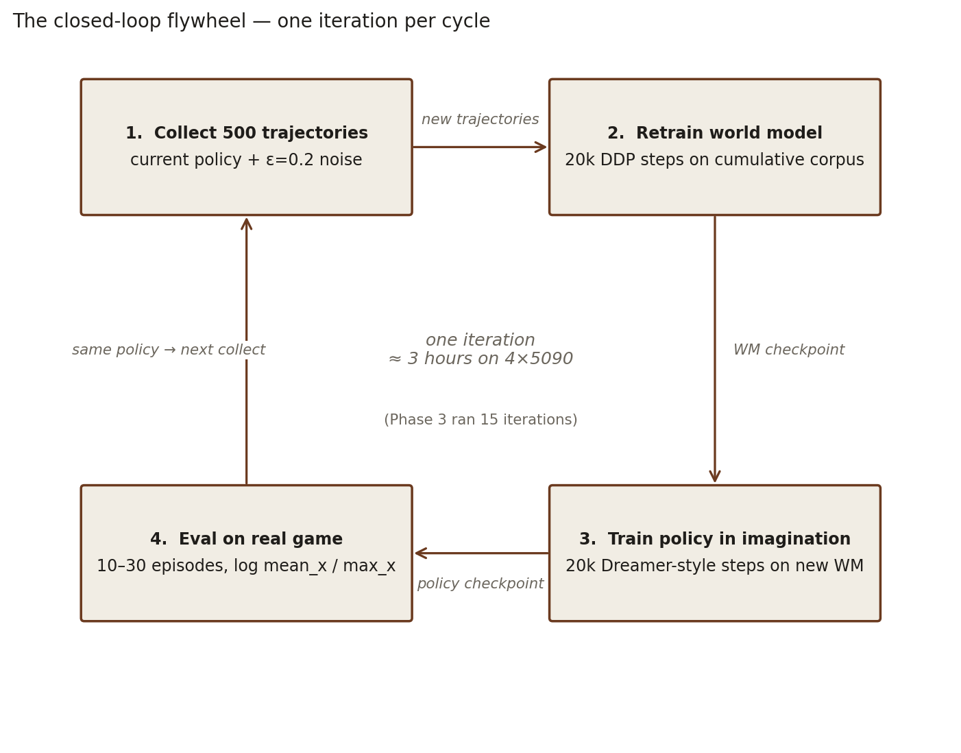
This is, in spirit, the Dreamer loop, with the LeWM constraint that the world model stays self-supervised — no reconstruction loss, no manually-engineered features, just the latent dynamics and the reward head bolted onto it.

What “training in imagination” actually means

Step 3 — “train a policy in imagination over the new world model” — is doing a fair amount of work in those few words. It’s the place the post’s eventual variance story lives, so it’s worth unpacking.

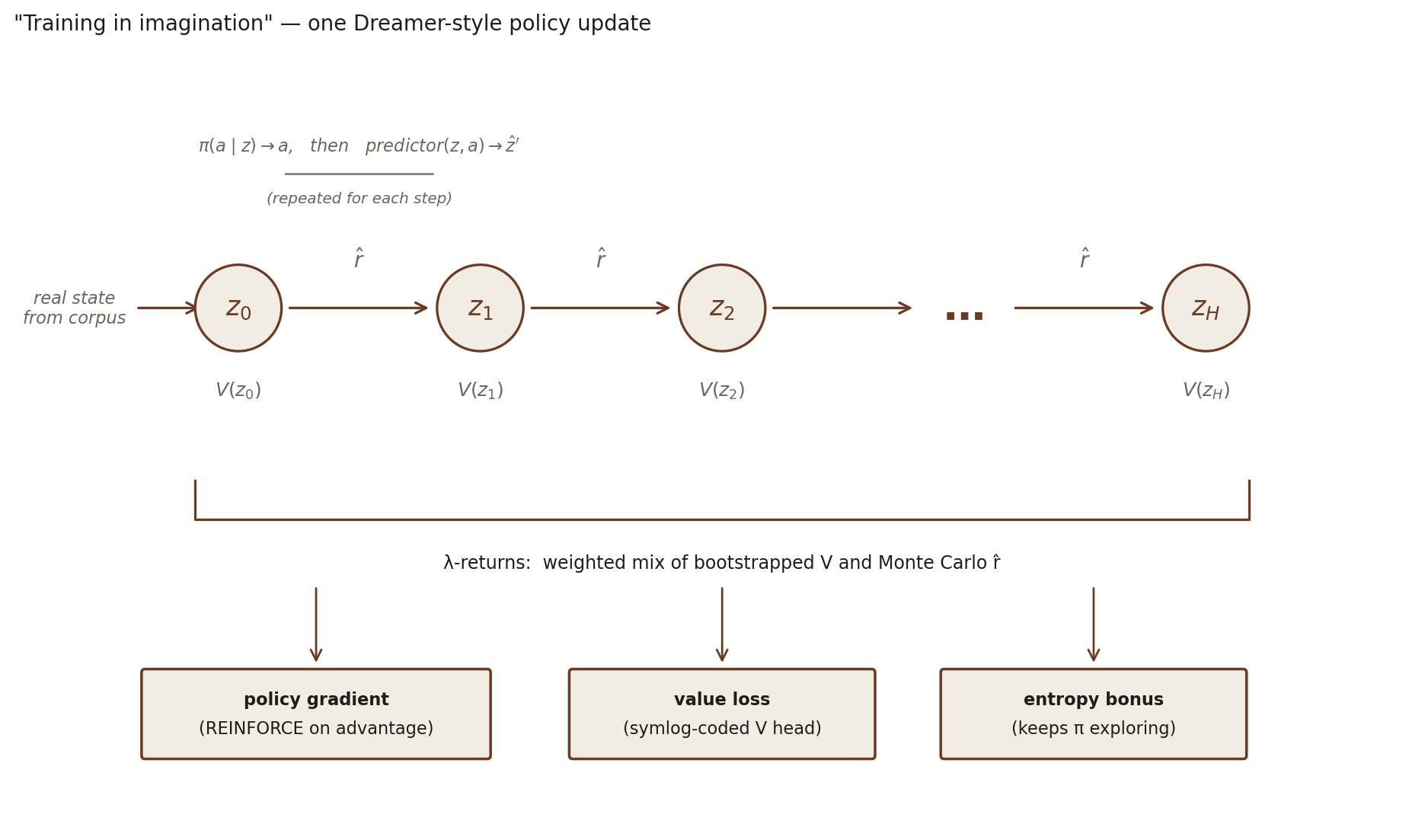
We use a Dreamer-v3-style setup: a stochastic policy π(a|z) maps latents to a distribution over Mario’s 12 buttons; a value head V(z) estimates expected long-run return from a latent. Both are small MLPs that operate over the frozen encoded latent. One training step works like this:

1. Sample real latents. Pull a batch of states the collector has actually visited — Mario at the spawn, mid-air, near a Goomba, at the entrance to a pipe — and encode them once.
2. Imagine forward H=15 steps. At each step the policy proposes an action, the predictor produces the next latent, the reward head produces a predicted reward, and the value head reads off an estimate of return from the new latent.
3. Compute λ-returns. A weighted mix of bootstrapped value estimates and Monte-Carlo predicted rewards, controlled by a λ hyperparameter (high λ = trust the chain of predicted rewards more; low λ = trust the value bootstrap more). The value head is symlog-coded — a Dreamer-v3 trick that squashes large returns into a stable target range, so the value loss isn’t dominated by occasional huge spikes from death penalties or score events.
4. Apply three gradients. Policy gradient (REINFORCE on the advantage = return − V), value loss (squared error against the symlog-coded return), and an entropy bonus that keeps π from collapsing onto a single button.

Nothing in this inner loop touches the real game. The policy improves by gradient-descending against the world model’s beliefs about consequences — which is exactly as reliable as the world model’s beliefs themselves are. That last clause becomes important.

The question we wanted to answer with the whole loop wasn’t “how fast does this converge?” It was “does it converge at all?“

05 · Fifteen iterations later

We ran fifteen iterations. Each one got a 10-episode stochastic eval on level 1-1, with the policy starting fresh from Mario at the spawn and 1500 frames of game time to make progress. Here is what those evals looked like.

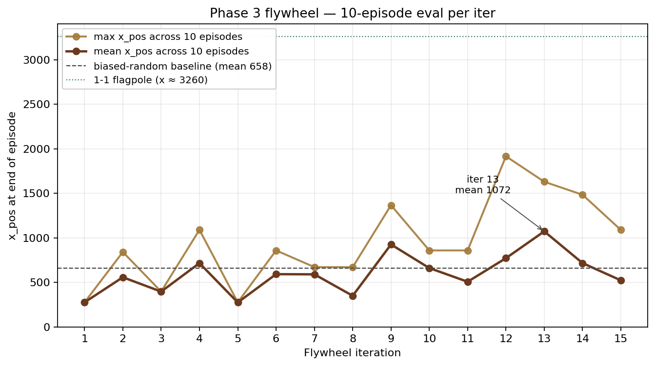
The visible pattern, if you trust each point, is dramatic. Iter 4 at mean 715 crosses the biased-random baseline (658) for the first time — the headline moment of the project. Iter 5, on a strictly better world model with a strictly larger corpus, immediately collapses back to 274, almost identical to the iter-1 score. Iter 6 partially recovers with a warm-start from iter 4. Iter 7 produces a 30-episode stochastic mean of 805 with a max of 1758 (the 10-ep CSV row in the plot above scored only 590 because random eval-seed luck put 7 of 10 episodes in a stuck mode the policy could only escape stochastically). Iter 9 is another breakthrough at 925. Iter 13 reaches mean 1072, max 1629 on the on-iter eval, and 30-episode stochastic eval at a different seed gave mean 1066 / max 1983 — the project’s best numbers anywhere. Iters 14 and 15 drop back to roughly 715 and 522.

Reading the line plot left-to-right, you’d write the story like this: a recipe that works, a fragile recovery, a slow climb, a peak, a regression. We did write that story — fifteen times. Each iter generated a tidy interpretation: time-cost regression, policy collapse, warm-start recovery, entropy-tuned breakthrough, corpus-quality regression. The interpretations were internally consistent. They were also, it turns out, mostly noise.

06 · The variance discovery

What broke the spell was iters 14 and 15. Two consecutive iters, no recipe change, no obvious training-time anomaly, both substantially below iter 13. The natural readings were cumulative corpus drift (the buffer was accumulating stuck-state frames) or catastrophic forgetting in the world model. Both made theoretical sense. Neither survived testing.

The first diagnostic was a frame-source audit. We grouped every frame in the buffer by which iter produced it and by which x_pos bucket its source trajectory reached, and computed the cumulative composition the world model saw at each iter:

Audit bucket	iter 12 share	iter 13 share	iter 14 share	iter 15 share
frames from trajectories that died at x < 200	0.2%	0.1%	0.1%	0.1%
frames from trajectories with max_x ∈ [200, 500)	8.4%	8.4%	8.1%	8.1%
frames from trajectories with max_x ∈ [500, 1000)	66.5%	65.7%	65.0%	64.5%
frames from trajectories with max_x ∈ [1000, 1500)	19.2%	19.3%	20.2%	20.6%
frames from trajectories with max_x ≥ 1500	5.7%	6.4%	6.5%	6.7%

Composition shifted by less than half a percentage point in every bucket between iter 13 and iter 14, and the trend on the far-progress (≥1500) bucket was up, not down. Whatever the iters 14–15 drops were, they weren’t cumulative corpus drift. We had to look elsewhere.

The second diagnostic was the one that actually answered the question. We took iter 13’s world model — the specific checkpoint the breakthrough came from — and trained five fresh policies on it with five different RNG seeds (100, 200, 300, 400, 500). Same buffer, same recipe, same hyperparameters, only the seed varied. Each got the same 30-episode stochastic eval.

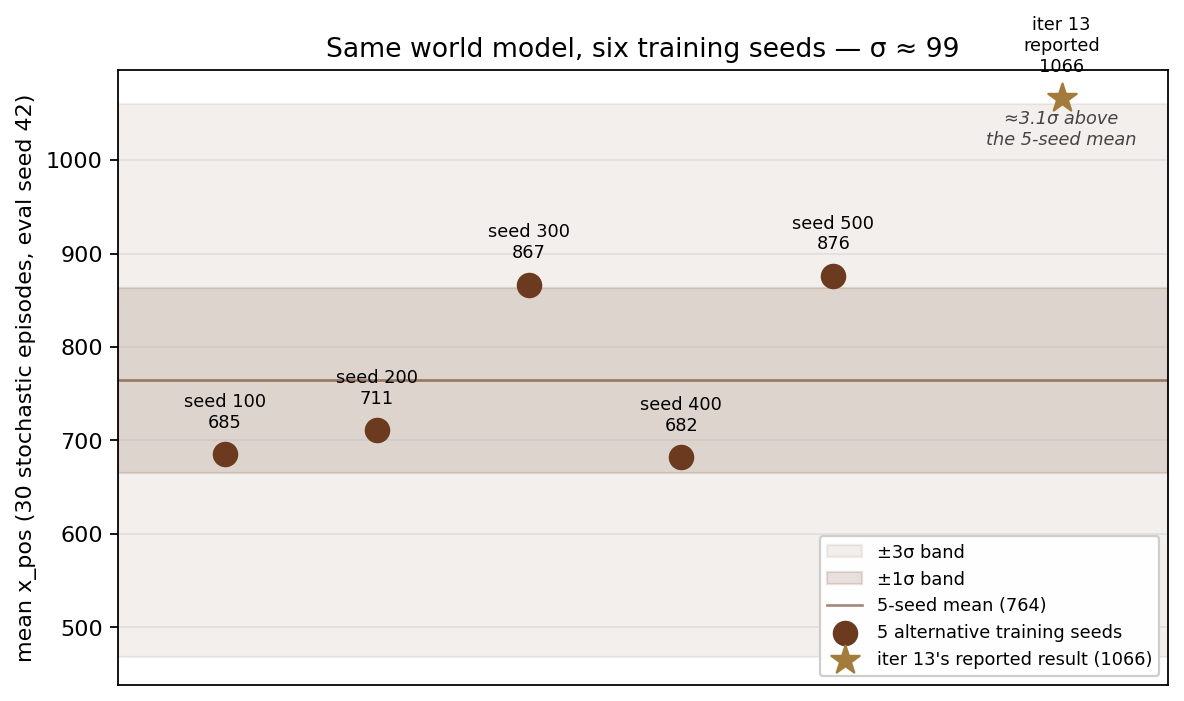
The five seeds spanned mean_x from 682 to 876, standard deviation 99. Iter 13’s reported 1066 is 3.06σ above the five-seed mean — a reproducible outlier, not a state of the world model. (Re-evaluating iter 13’s saved policy at the same eval seed scored 1066 again, ruling out evaluation noise as the explanation.) Seed 400 mode-collapsed: every one of its 30 episodes terminated at exactly x = 682, the same stuck spot, with no exploration ever finding an exit. That failure mode is invisible to a single-seed eval — you’d just see a low mean and not know whether it was bad training or a degenerate distribution.

What this means for the iter-by-iter story is uncomfortable. Iter 13’s breakthrough wasn’t a property of the world model. It was a property of the seed-zero training run on that world model. Iter 14’s “regression” was a typical draw from the same distribution. Iter 5’s “collapse” might have been a typical draw. So might iter 8’s, iter 11’s, iter 12’s bimodality. We can’t decisively re-label each one — we’d need K-seed data for every iter — but we can say that a difference of 200 points between two consecutive iters carries less information than we treated it as carrying. The flywheel did not have a regression problem. It had a single-sample-per-iter problem.

07 · Two recipe failures, both invisible at training time

Before this, the project had already eaten one expensive lesson in the same family. The first few hundred hours of H3 work — the entire reward-augmented JEPA arc that produced the early world-iter* and policy-iter* checkpoints — was conducted over a world model whose predictor had silently collapsed to a constant output. A gradient explosion in the unnormalized MLP predictor triggered the dying-GELU pathology: most of the predictor’s hidden units saturated at zero gradient and stayed there, leaving the final linear layer to emit roughly final_linear.bias regardless of input. The encoder was fine. The reward head fit. The training curves looked clean — loss descended, val tracked train. The only signal that anything was wrong was the value the loss converged to, which roughly equalled the variance of the latents under no conditioning. That’s a signal you can only read if you already suspect the result.

We caught it by sweeping inputs at fixed seed and watching the predictor’s output not move. The fix was a residual + LayerNorm predictor (we call this V2). Every “phase 3” result on this site is over V2. Everything before it, we discarded.

These two failures rhyme.

When a training-time diagnostic says everything is fine and a downstream number tells a clean story, the diagnostic might still be wrong and the story might still be noise.

In the predictor-collapse case, the diagnostic was the training loss — descending, stable, low. The story was “reward-augmented JEPA works.” The reality was a 124M-parameter constant function.

In the variance case, the diagnostic was the per-iter real-env eval — bouncing around, sometimes high, sometimes low. The story was “iter 4 breakthrough, iter 5 collapse, iter 13 peak, iter 14 regression.” The reality was a sequence of independent draws from a wider distribution than we’d ever measured.

Both failures share the same shape: a downstream metric was being interpreted one sample at a time, and the underlying noise was wider than the differences the interpretation depended on. There’s a similar lesson lurking in our SSL transfer experiments — rank-orders that depend on two-point training curves, or on small held-out sets, flip with the next random seed. We knew that one. We did not connect it to RL training variance until the iter-13 diagnostic pinned it down.

08 · What we’re building next — Flywheel v2

The fix is structural. Single-sample evals are the input to every operator decision the flywheel makes; if they’re noisy, every decision is noisy. The new design — we’re calling it Flywheel v2 — has four mechanisms.

M1 — K-seed policy training per iter. Instead of training one policy on each iter’s world model, we train K=4 policies in parallel — one per GPU, seeds iter * 1000 + {1, 2, 3, 4}. Each gets the same 30-episode stochastic eval. The best by mean x is kept as the iter’s official policy artifact; the full K-tuple of scores is logged. This is a direct response to the diagnostic: the per-iter signal becomes the mean-of-K with measured stdev, not a single draw. Best-of-4 over a σ=99 distribution puts the on-iter score reliably in the 850–950 band rather than the 600–1000 band. The K=4 evals also let us measure the iter’s stdev in situ — so we know how much signal we have without running a separate diagnostic. And per-seed mode collapse (one policy converging to a stuck-state) becomes visible automatically, not hidden inside a low mean. The compute cost is roughly 4× policy training, but policy training is the cheap part of an iter (the world model dominates). End-to-end wall time goes from ~3 hours to ~3.5 hours.

M2 — Hall of fame. Every iter, the (world model, policy, eval results) triple is copied — not symlinked — into checkpoints/hof/iter{N}_meanx{mean}_maxx{max}/, with a JSON catalog indexed by score. Nothing ever gets overwritten by a later iter. This means recovery from a bad iter is just a path change; warm-starts can come from the top-K of the catalog rather than the most recent iter; and ensemble inference over multiple HOF world models becomes possible (not v2’s default, but enabled by the storage). Each entry is about 200 MB, so 100 iters is 20 GB — trivial against the 26 GB of corpus.

M3 — Bounded stratified replay buffer. The current corpus is append-only and frame-uniform-sampled. Both choices have been load-bearing in the wrong direction. One stuck trajectory contributes ~1500 frames (Mario stands at x=50 for the whole rollout); one death contributes ~50; the audit-table tier of 65% [500, 1000) frames absorbs most of the world model’s training gradient regardless of how representative those states are. v2 replaces this with a 5,000-trajectory buffer, stratified by source-tier and capped on frame share, not trajectory count. The Elite tier (max_x ≥ 1500) is unbounded; the Stuck tier (200 ≤ max_x < 700) is capped at 30% of corpus frames.

M4 — Improvement detector. With M1 giving us per-iter stdev, the question “did this iter improve over the previous best?” becomes a statistical test, not an editorial decision. The detector emits one of three outcomes after each iter — commit, branch (run a recovery iter with one variable flipped), or halt (operator intervention required). The 1σ threshold uses M1’s measured stdev, not a global constant, so the rule adapts as we get more reliable.

Phase A of the v2 rollout is M1 + M2. We expect to ship it in the next day or two; the diagnostic script the reliability test was built on (scripts/diag_iter13_variance.sh) already runs the parallel-seeds pattern, so the wiring change is small. M3 and M4 come after we’ve validated that M1 actually does what the variance math says it should.

09 · Where this leaves things, and what we’d like to see

We have a self-supervised world model that linearly probes to the game’s internal physics, a closed-loop training pipeline that produces policies clearing more than half of level 1-1, and a recently-arrived appreciation that none of our per-iter measurements have been quiet enough to use. The pipeline works; the instrumentation didn’t, and that’s the thing v2 fixes.

A few things we want to know once Flywheel v2 is running, in roughly decreasing order of how much we expect them to surprise us:

• Does measured per-iter stdev actually drop to ~30 under M1? The statistics say it should. If it doesn’t, the variance source isn’t policy training and we’re chasing the wrong knob — a possible candidate is variance in world-model training itself, which we have not measured.
• Does the HOF catalog reveal monotone improvement that the noisy per-iter scores hid? A clean rising plot of HOF-best across iters is the cleanest possible evidence that the underlying system was improving and we were just unable to see it.
• What’s the actual per-level transfer story? Today’s policy is trained on level 1-1 only. The model has the architectural pieces to take a level identifier as input; the curriculum work is in v2’s later phases (M3 + buffer-per-level), but the first multi-level eval will tell us how far the 1-1 features generalize off-distribution.
• Where does the flagpole live? The best run anywhere in the project (a filtered-corpus side experiment with max_x = 2719) gets about 83% of the way to the 1-1 flagpole. We don’t yet know whether the remaining 540 pixels are a recipe gap, a representation gap, or a long-tail-of-screen-states gap. Probably all three.

The clip at the top of this post is one of thirty stochastic episodes from iter 13 — a single draw, the best we have, with no claim to being representative. That uncertainty is the whole reason we’re pausing iter-tuning to rebuild the measurement layer instead of pushing on to iter 16.

---

Lemario builds on open work by the JEPA and LeWorldModel teams at Meta AI, the authors of gym-super-mario-bros and nes-py, and SethBling, whose MarI/O remains the project’s point of comparison. Thanks to all of them.